A crash map can reveal where incidents have accumulated, but location alone cannot explain why some parts of a city report more crashes than others. Regression provides a way to test whether crash counts tend to vary alongside characteristics such as road type, recorded speed limits, construction-zone activity, population density, or household income.
Spatial regression adds another question: are those relationships consistent across a city, or do they change from one area to another? This project compared two regression approaches:
- Ordinary Least Squares (OLS) estimates one citywide relationship between each explanatory variable and the outcome.
- Geographically Weighted Regression (GWR) estimates local relationships, allowing the modeled coefficients to vary across space.
Comparing the two approaches helped determine whether a single equation could adequately describe Austin’s crash patterns or whether those relationships changed across the city.
This analysis focused on Austin, Texas. The U.S. Census Bureau estimated that Austin had 993,588 residents in 2024, making it the 13th-most populous city in the United States. Its size, varied road network, and mixture of dense urban and lower-density areas made it a useful setting for examining whether one statistical model could adequately describe crash patterns across the entire city.
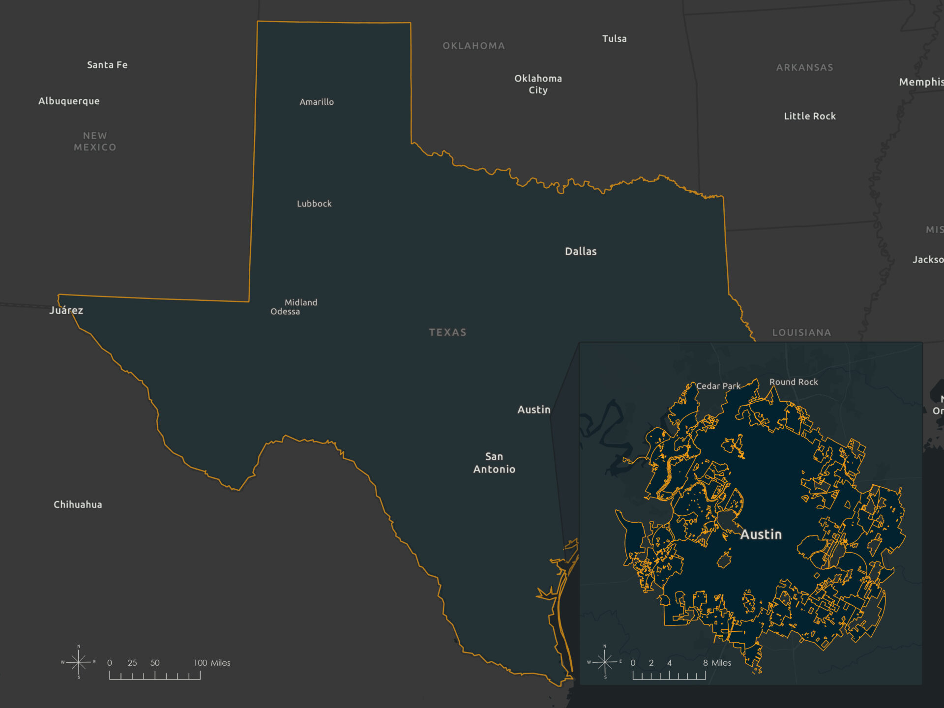
The project compared a global Ordinary Least Squares (OLS) model with a local Geographically Weighted Regression (GWR) model. ArcGIS Pro was used for spatial data preparation, exploratory regression, OLS, residual spatial-autocorrelation testing, GWR, and cartography. R in RStudio was used to visualize variable distributions and model residuals. The objective was exploratory: to identify promising relationships, evaluate whether the statistical assumptions held, and determine whether those relationships appeared to vary across Austin.
Building the tract-level dataset
Crash records from the City of Austin were combined with road, demographic, and boundary data. All spatial data were downloaded on August 7, 2025, clipped to the Austin jurisdictional boundary, and projected to NAD 1983 StatePlane Texas Central FIPS 4203 Feet.
| Layer | Source | Dataset or service | Variables used |
|---|---|---|---|
| Crash incidents | City of Austin Open Data Portal | Austin Crash Report Data: Crash Level Records | Cumulative crash count; mean crash-record speed limit; construction-zone crash percentage |
| Roads | U.S. Census Bureau | TIGER/Line Roads for Travis county | Primary-road mileage percentage |
| Median household income | Esri | ACS Median Household Income Variables: Boundaries | Median household income |
| Census tracts | Esri | USA Census Tract Boundaries | Population density and analysis units |
| Austin jurisdiction | City of Austin Open Data Portal | BOUNDARIES jurisdictions | Study-area boundary |
The final analysis used 295 census-tract features intersecting the Austin jurisdictional boundary. Summarizing the data to a common geographic unit made it possible to compare the variables consistently, although it also generalized street-level differences within each tract.
The dependent variable was:
- Cumulative reported crash count: The number of reported crashes recorded in each tract between January 2010 and July 2025.
Five candidate explanatory variables were evaluated:
- Mean posted speed limit among recorded crashes: The average posted speed limit stored with crash records in each tract. This represents conditions associated with reported crashes, not the average speed limit across the tract’s entire road network.
- Primary-road mileage percentage: The percentage of mapped road mileage classified as an Interstate, U.S. Route, or State Route using TIGER/Line road-type codes.
- Population density: The estimated number of residents per square mile in 2023.
- Construction-zone crash percentage: The percentage of reported crashes identified as occurring in a construction, maintenance, or utility work zone.
- Median household income: The estimated median annual household income for each census tract.
Two of these variables, mean posted speed limit and construction-zone crash percentage, were calculated from the crash records themselves. They describe characteristics associated with recorded crashes rather than independently measured roadway exposure. Relationships involving these variables should therefore be interpreted as exploratory associations.
Mapping the variables before modeling revealed that each followed a different spatial pattern. Crash counts and crash-related variables tended to emphasize transportation corridors, while population density and household income described broader neighborhood conditions.
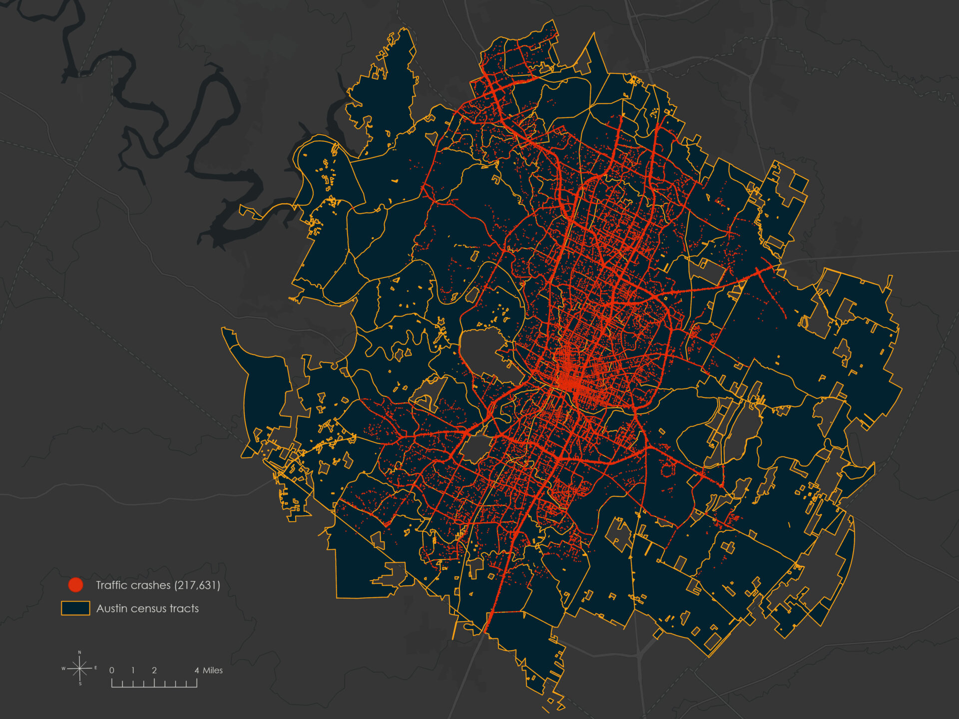
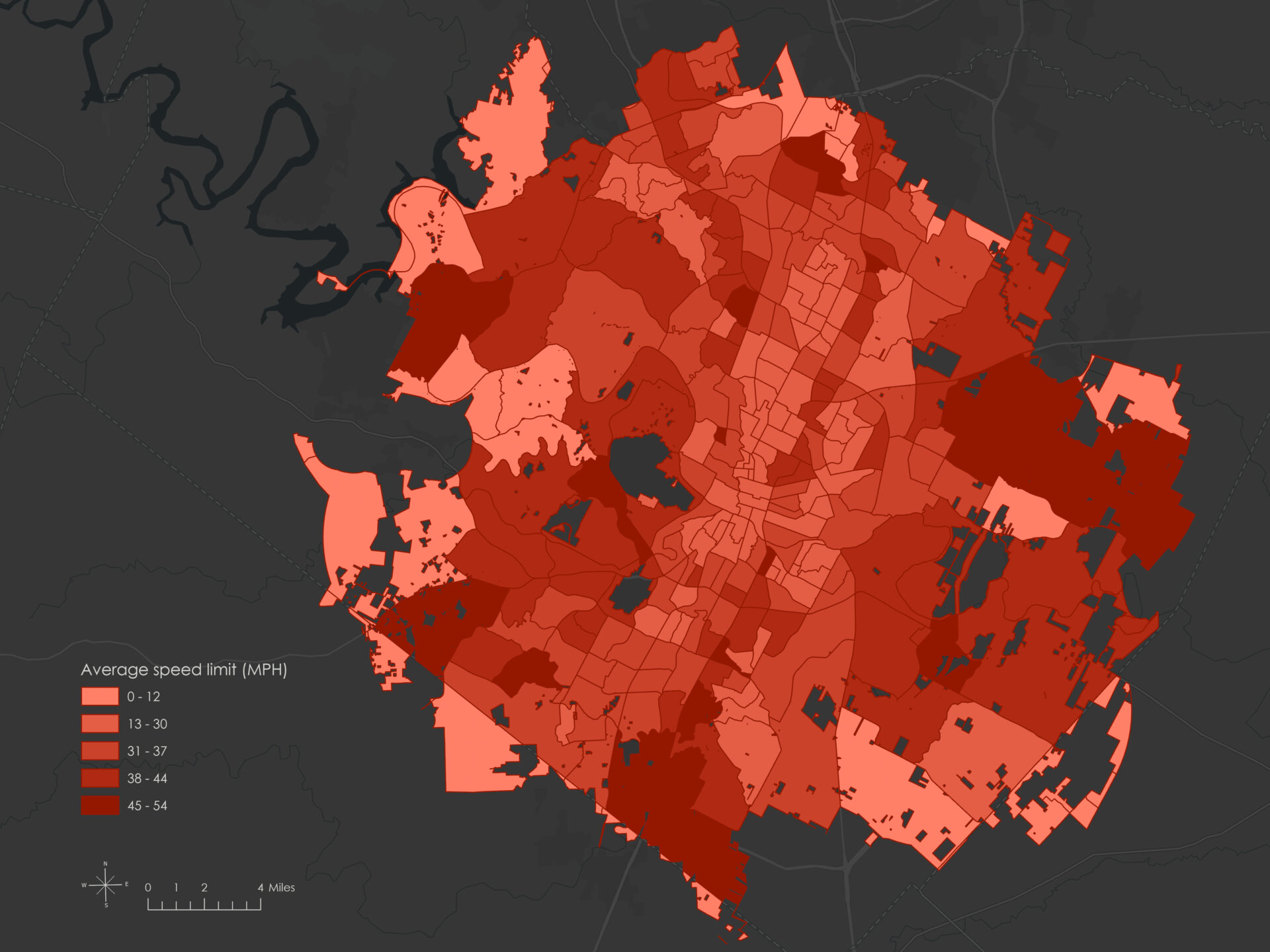

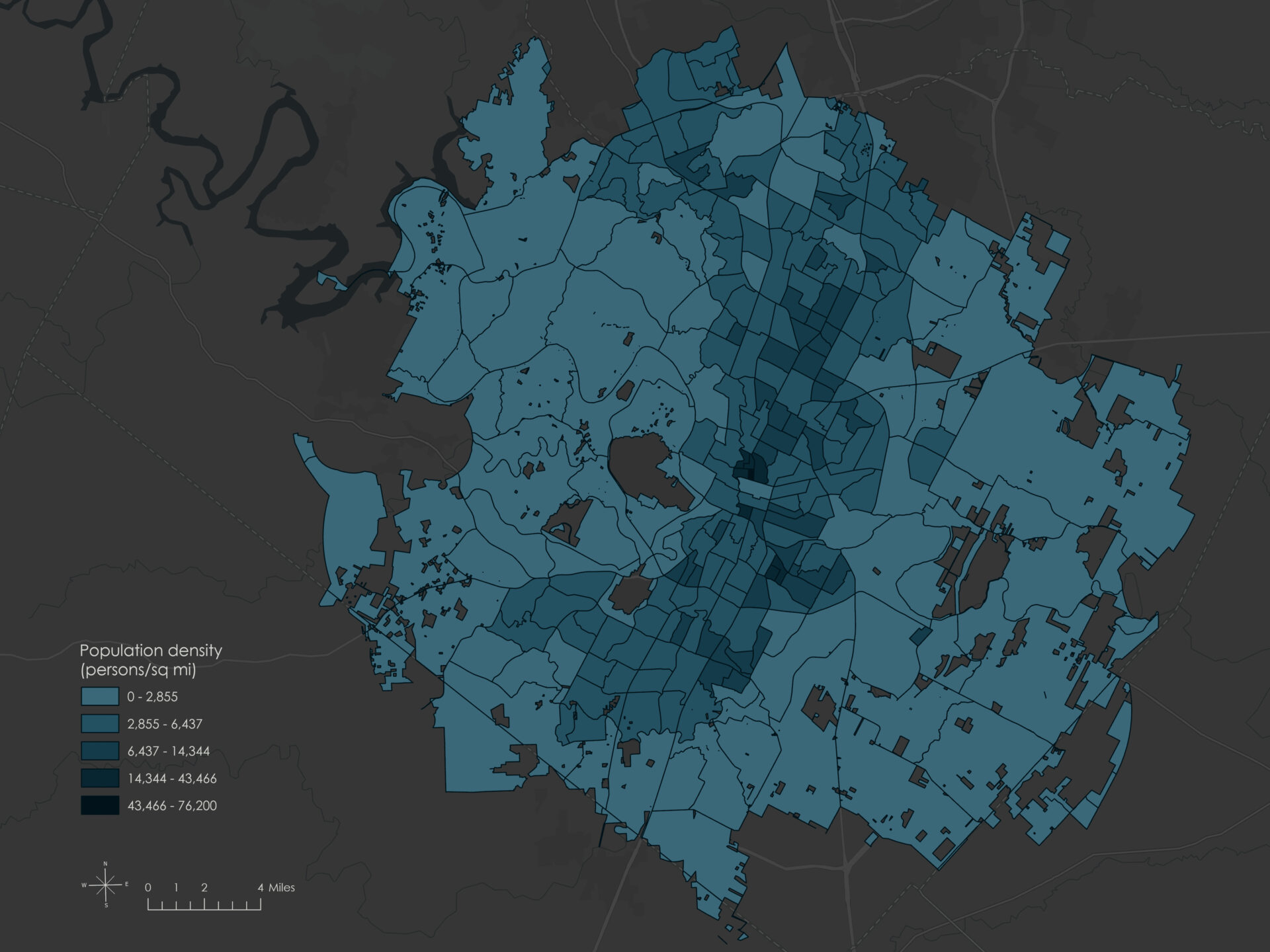
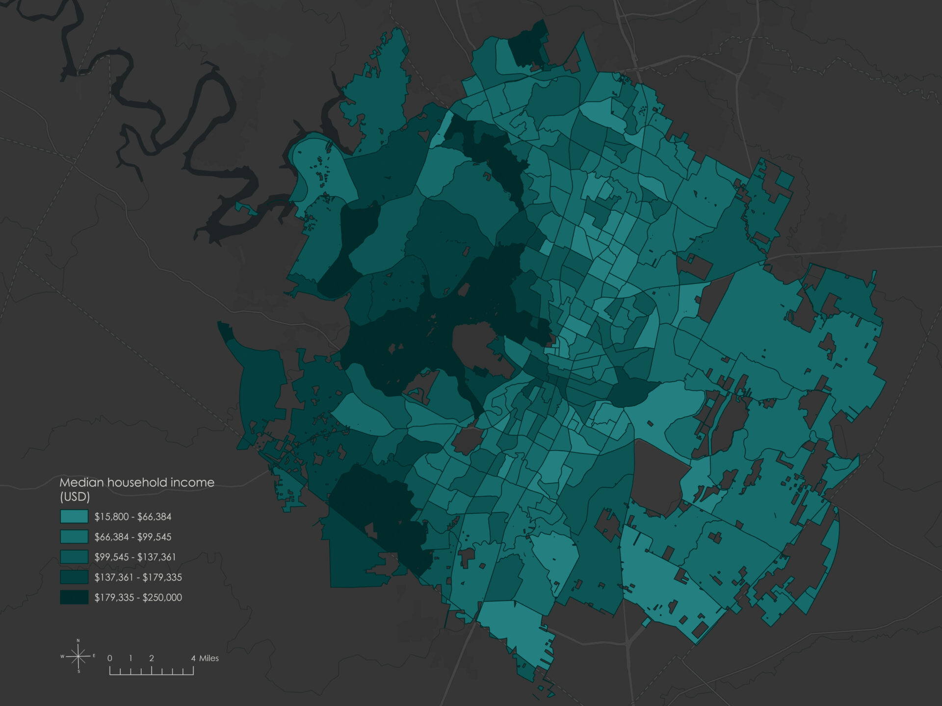
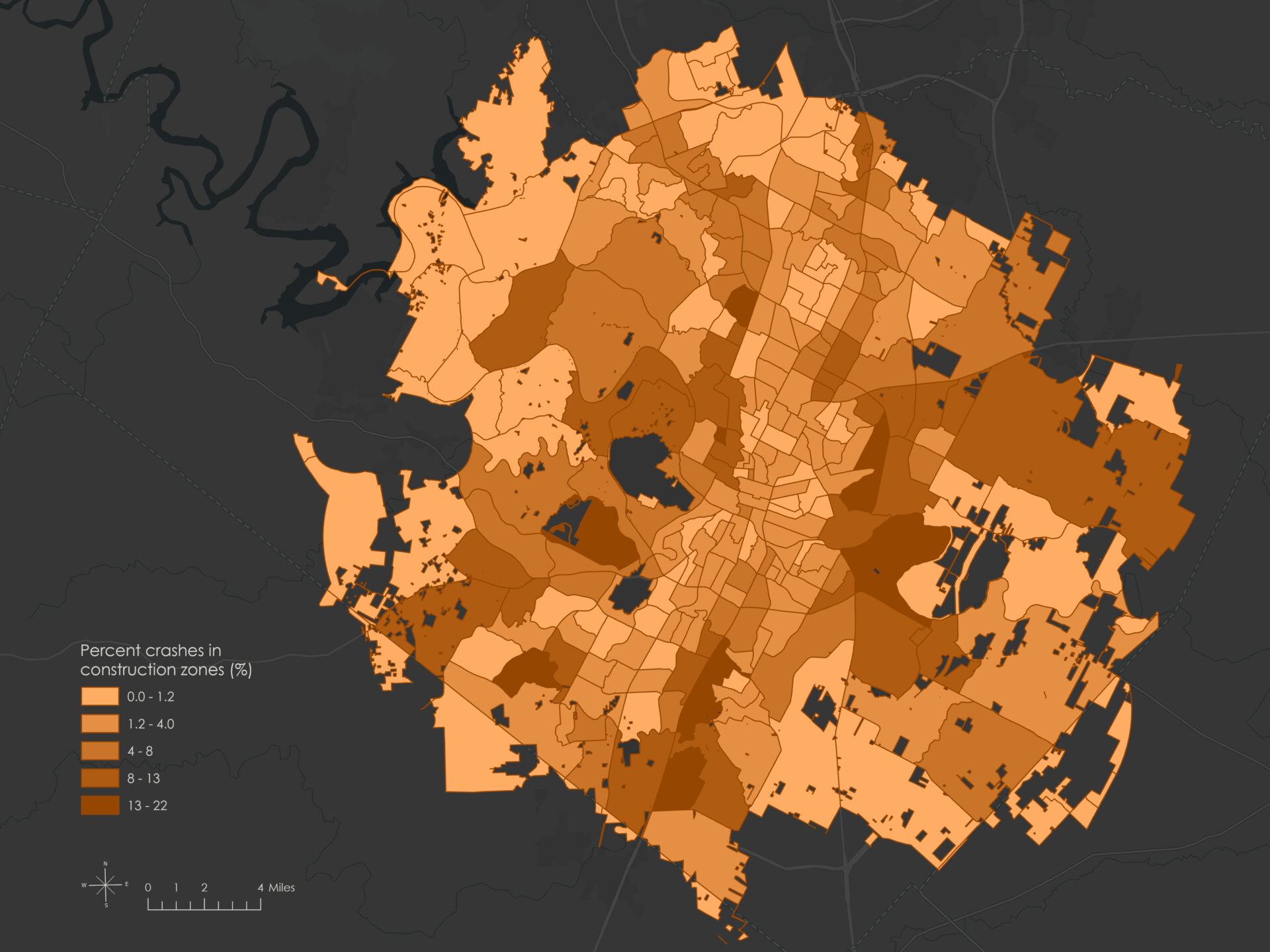
Null values were replaced with zero only where a missing value was interpreted as the absence of a mapped feature or recorded event, such as no primary-road mileage or no recorded crashes. Because an unrecorded value does not always mean that a feature was absent, this assumption is an important limitation.
Searching for a global explanation
Exploratory Regression tested combinations of the five candidate explanatory variables using OLS. The purpose was to identify a promising global model while screening for excessive predictor redundancy, poorly distributed residuals, inconsistent variance or relationships, and unexplained spatial clustering.
The search used a target adjusted R² of 0.50 and a maximum Variance Inflation Factor (VIF) of 7.5. Adjusted R² measures model fit while accounting for the number of variables, and VIF helps identify explanatory variables that contain highly redundant information.
No tested model met all of the screening criteria. The strongest candidate contained mean crash-record speed limit, median household income, and construction-zone crash percentage.
| Adjusted R² | AICc | Jarque-Bera p | Koenker p | Maximum VIF | Moran’s I p | Candidate model |
|---|---|---|---|---|---|---|
| 0.25 | 4,643.37 | <0.001 | 0.01 | 1.40 | <0.001 | + Mean crash-record speed limit− Median household income+ Construction-zone crash percentage |
This candidate accounted for approximately one-quarter of the tract-level variation in crash counts after accounting for model complexity. Its VIF values provided little evidence of problematic redundancy among the three variables, and its AICc was the lowest among the tested models. AICc compares models while penalizing unnecessary complexity, with lower values indicating better relative fit.
However, the model did not reach the adjusted R² target and failed several diagnostic tests:
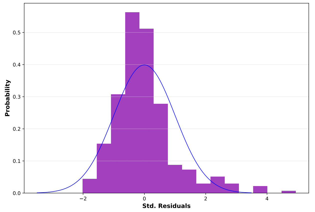
- The significant Jarque-Bera test indicated that the residuals departed from a normal distribution.
- The significant Koenker test indicated that the variability of the residuals, the modeled relationships, or both were not consistent across the study area.
- The significant Moran’s I test indicated that the model’s errors remained spatially clustered.
The result was therefore useful as a candidate for closer examination, not as a fully specified explanatory model.
OLS was then run separately using the three selected variables. OLS estimates one coefficient for each variable and applies that relationship across every tract in Austin.
| Variable | Coefficient | Standard error | t-statistic | Standard p | Robust standard error | Robust t | Robust p | VIF |
|---|---|---|---|---|---|---|---|---|
| Intercept | 445.009522 | 127.158847 | 3.499635 | <0.001 | 87.330086 | 5.095718 | <0.001 | n/a |
| Mean crash-record speed limit | 18.673691 | 3.110208 | 6.004002 | <0.001 | 2.599931 | 7.182380 | <0.001 | 1.403958 |
| Median household income | −0.003159 | 0.000799 | −3.956042 | <0.001 | 0.000631 | −5.006675 | <0.001 | 1.022640 |
| Construction-zone crash percentage | 20.553942 | 10.261864 | 2.002944 | 0.046 | 11.204707 | 1.834402 | 0.068 | 1.395238 |
Because the Koenker test was significant, the robust probabilities provide the safer basis for evaluating the coefficients. Mean crash-record speed limit and median household income remained statistically significant under the robust estimates. Construction-zone crash percentage had a conventional p-value of 0.046 but a robust p-value of 0.068, so it did not remain significant at the 0.05 level after the robust adjustment.
These coefficients represent statistical associations within this dataset, not evidence that any variable caused crashes. That distinction is especially important for the speed-limit and construction-zone measures because both were derived from the crash records.
The Joint Wald statistic was significant at p < 0.01, indicating that the explanatory variables were jointly associated with crash counts. That result did not override the evidence of non-normal, nonconstant, and spatially clustered residuals.
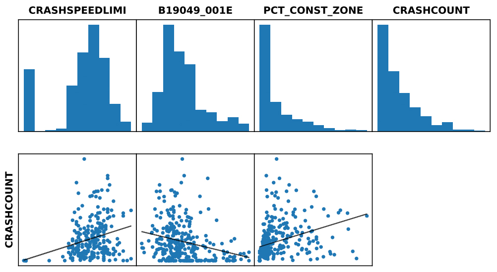
The supporting plots reinforce the diagnostic results. Crash counts and several explanatory variables were unevenly distributed, and the relationships were not adequately summarized by clean linear trends.
Testing what the global model missed
A residual is the difference between an observed value and the value predicted by a model. If a global regression is working well, large positive and negative residuals should not form a systematic geographic pattern. Clusters of similar residuals suggest that the model is repeatedly underpredicting or overpredicting in particular parts of the city.
The OLS residuals were tested using Global Moran’s I with Euclidean distance and inverse-distance weighting. The result produced a Moran’s I of 0.149, a z-score of 7.59, and a p-value below 0.0001.
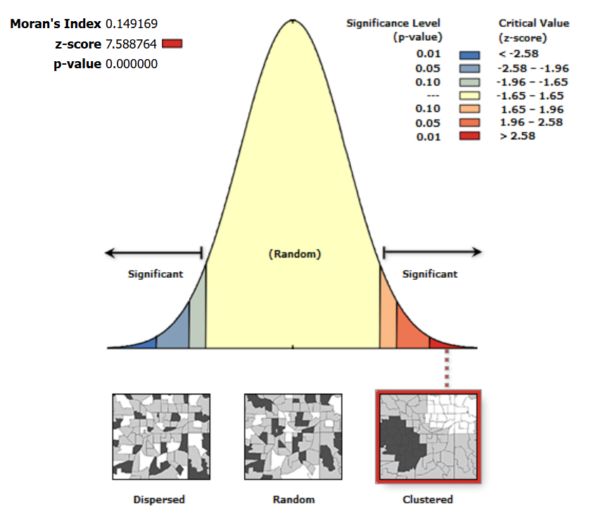
This clustering did not identify the cause of the model errors, but it showed that those errors were spatially organized. A single citywide equation was systematically missing something about where crashes accumulated, how the selected variables behaved, or both.
Allowing relationships to vary across Austin
Geographically Weighted Regression addresses spatially varying relationships by estimating a local regression equation for each feature. Nearby observations contribute more to a tract’s local estimate than distant observations, allowing coefficients to change across the study area.
The GWR model used the same three variables as the OLS model:
| Model setting | Value |
|---|---|
| Number of features | 295 |
| Dependent variable | Cumulative reported crash count |
| Explanatory variables | Mean crash-record speed limit Median household income Construction-zone crash percentage |
| Neighborhood | 69 neighbors |
The GWR model produced a lower AICc and higher R² values than the global model.
| Metric | GWR | OLS |
|---|---|---|
| R² | 0.5527 | 0.2563 |
| Adjusted R² | 0.4400 | 0.2486 |
| AICc | 4,592.97 | 4,643.37 |
| Effective degrees of freedom | 235.82 | n/a |
| Sigma-squared | 291,584 | n/a |
The GWR AICc was approximately 50 points lower than the OLS value. Because AICc accounts for model complexity, that difference supports the conclusion that the local model fit these observations better than the global model.
The unadjusted GWR R² was 0.5527, while the adjusted R² was 0.44. Reporting both values is important because a local model estimates many more relationships than a global one. The improved fit supports exploring spatial variation, but it does not validate the model, demonstrate causation, or show that all important crash-related variables were included.
The mapped local coefficients illustrate how the estimated relationships changed across Austin. Positive coefficients indicate that higher values of a variable were associated with higher modeled crash counts in that area. Negative coefficients indicate an inverse association, while values near zero indicate a weaker estimated relationship.
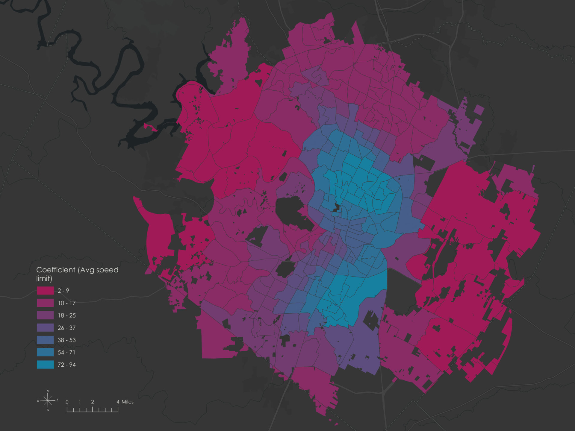
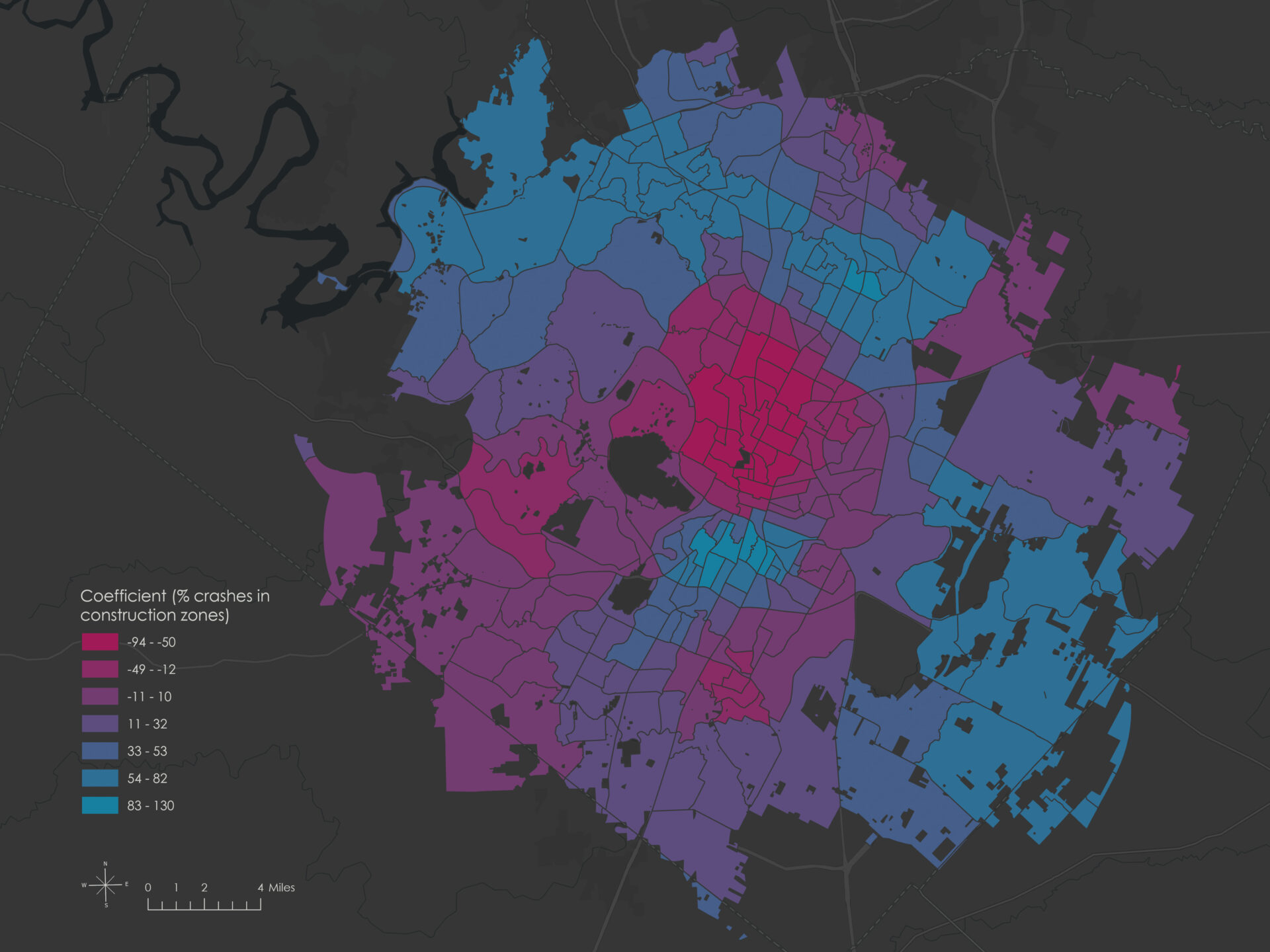
These maps do not establish that the variables had statistically significant effects in every tract. Instead, they demonstrate the central value of the local model: relationships that appeared uniform in a global coefficient became geographically varied when estimated across the city.
What the models explain and what they miss
The global analysis identified a useful candidate model, but its modest fit and failed residual diagnostics showed that a single equation did not adequately describe Austin’s crash pattern. GWR fit the observations better according to AICc and revealed substantial geographic variation in the estimated coefficients. Together, the results suggest that the relationships captured by these variables were not constant across the city.
The findings should nevertheless be treated as exploratory indicators. Several limitations affect their interpretation:
- The dependent variable was a cumulative crash count covering more than 15 years. It was not normalized by traffic volume, vehicle miles traveled, or another direct measure of roadway exposure.
- The crash, road, population, and income data did not all represent the same time period. Recent demographic estimates may not describe conditions throughout the full 2010–2025 crash-record period.
- Mean speed limit and construction-zone percentage were derived from crash records rather than independent inventories of roadway conditions. They describe the recorded crashes as much as they describe the tracts.
- Census-tract aggregation conceals differences among individual streets and intersections. The results also depend on the locations and sizes of the tract boundaries used.
- The crash-count distribution was strongly skewed, and the OLS model did not satisfy several important assumptions. A count-based model, such as a Poisson or negative-binomial spatial model, would be worth evaluating in future work.
- Replacing null values with zero assumes that missing records indicated the absence of a feature or event. That assumption may not hold where the source data were incomplete.
- Important explanatory variables were unavailable, including traffic volume, intersection density and design, road geometry, land use, time-specific construction activity, and temporal crash patterns.
The diagnostics revealed when a single citywide equation was insufficient, and the local model translated that limitation into a geographic pattern. The most useful result is not a definitive list of crash causes, but a clearer framework for asking where relationships differ across Austin and what additional evidence would be needed to explain them.
Citations
City of Austin. (n.d.-a). Austin crash report data: Crash level records [Data set]. Austin Open Data Portal. https://data.austintexas.gov/Transportation-and-Mobility/Austin-Crash-Report-Data-Crash-Level-Records/y2wy-tgr5/about_data
City of Austin. (n.d.-b). BOUNDARIES_jurisdictions [Data set]. Austin Open Data Portal. https://data.austintexas.gov/dataset/BOUNDARIES_jurisdictions/3pzb-6mbr
City of Austin Transportation and Public Works Department. (n.d.). Vision Zero viewer [Interactive map]. https://visionzero.austin.gov/viewer/
Esri. (n.d.-a). ACS median household income variables: Boundaries [Feature layer]. ArcGIS Online. https://www.arcgis.com/home/item.html?id=45ede6d6ff7e4cbbbffa60d34227e462
Esri. (n.d.-b). How geographically weighted regression works [ArcGIS Pro documentation]. https://pro.arcgis.com/en/pro-app/latest/tool-reference/spatial-statistics/how-geographicallyweightedregression-works.htm
Esri. (n.d.-c). How OLS regression works [ArcGIS Pro documentation]. https://pro.arcgis.com/en/pro-app/latest/tool-reference/spatial-statistics/how-ols-regression-works.htm
Esri. (n.d.-d). Interpreting exploratory regression results [ArcGIS Pro documentation]. https://pro.arcgis.com/en/pro-app/latest/tool-reference/spatial-statistics/interpreting-exploratory-regression-results.htm
Esri. (n.d.-e). USA Census tract boundaries [Feature layer]. ArcGIS Online. https://www.arcgis.com/home/item.html?id=20f5d275113e4066bf311236d9dcc3d4
U.S. Census Bureau. (2024). 2024 TIGER/Line shapefiles: Roads [Data set]. https://www.census.gov/cgi-bin/geo/shapefiles/index.php?year=2024&layergroup=Roads
U.S. Census Bureau. (2025, May 15). Population growth reported across cities and towns in all U.S. regions [Press release]. https://www.census.gov/newsroom/press-releases/2025/vintage-2024-popest.html
Categories: Mapping, Spatial data management, Spatial analysis, Scripting and development