On June 17, 2024, lightning ignited the South Fork Fire on the Mescalero Apache Reservation near Ruidoso, New Mexico. Driven by high winds, the fire expanded to more than 15,000 acres within its first 24 hours and prompted the evacuation of Ruidoso. Its final reported extent was 17,569 acres, or approximately 7,110 hectares, and incident reports estimated that roughly 1,400 structures were lost in the affected area.
A fire perimeter shows where a wildfire traveled, but it does not show how evenly the landscape burned. Burn severity estimates the magnitude of change to vegetation, soil, and other surface conditions by comparing spectral reflectance before and after a fire. This analysis used that change to examine where the South Fork Fire produced its strongest surface effects, how the mapped burn pattern varied among land-cover classes, and where burned areas overlapped populated parts of the region.
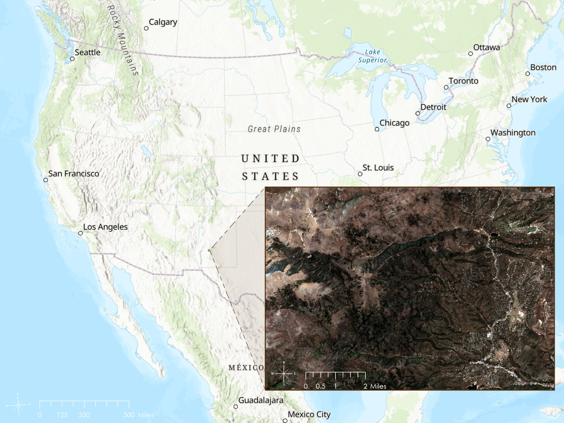
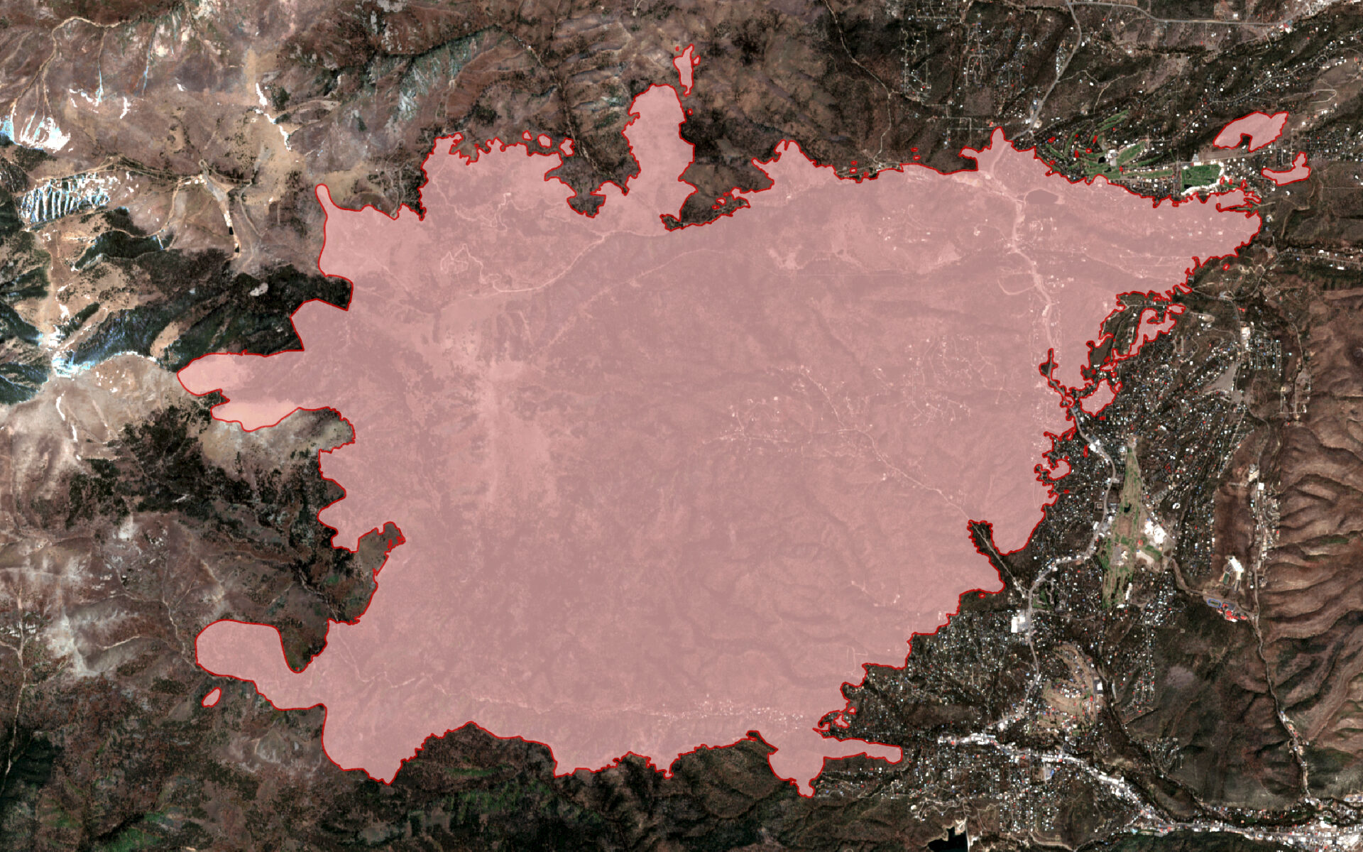
The nearby Salt Fire also began on June 17, burning south of Ruidoso at the same time as the South Fork Fire. Separating the two incidents was important because combining their spectral effects would have distorted the before-and-after comparison. At the time of the analysis, the South Fork Fire was too recent to appear in the Monitoring Trends in Burn Severity archive, so I obtained the best-available incident perimeter from the National Interagency Fire Center’s WFIGS Current Interagency Fire Perimeters service.
The workflow moved between Google Earth Engine, RStudio, and ArcGIS Pro. Google Earth Engine provided access to the satellite collections and supported the creation of cloud-filtered image composites and derived raster products. RStudio was used for statistical summaries and charts, while ArcGIS Pro supported raster assembly and final cartographic design.
| Data | Source | Analytical role |
|---|---|---|
| Fire perimeter | NIFC WFIGS Current Interagency Fire Perimeters | Defined the South Fork Fire study area |
| Satellite imagery | Harmonized Sentinel-2 MSI Level-2A | Created pre- and post-fire composites and vegetation indices |
| Active-fire detections | NASA FIRMS | Provided context for the active-fire period |
| Land cover | Dynamic World V1 | Supported exploratory comparisons among land-cover classes |
| Population | Global Human Settlement Layer | Estimated modeled population within mapped burned areas |
| Watersheds | HydroSHEDS | Provided regional hydrologic context |
Building a before-and-after view
The analysis began with two Harmonized Sentinel-2 image collections. The pre-fire collection covered June 16, 2023, through June 16, 2024, while the post-fire collection covered August 27 through October 31, 2024. The longer pre-fire window increased the pool of usable observations; the post-fire window captured conditions after the active-fire period while limiting, though not eliminating, the influence of early vegetation regrowth.
Both collections were filtered to the study area and to scenes with less than 1 percent cloud cover. An additional mask removed cloud, cloud-shadow, and invalid pixels using the Sentinel-2 scene-classification band. Reflectance values were scaled, and a per-pixel median was calculated across each collection to reduce residual clouds and other temporal noise.
The following excerpt illustrates how the image collections and median composites were created in Google Earth Engine:
// Create pre-fire image collection
var prefireRawImCol = ee.ImageCollection(
    "COPERNICUS/S2_SR_HARMONIZED"
  )
  .filterDate('2023-06-16', '2024-06-16')
  .filterBounds(roi)
  .filterMetadata(
    'CLOUDY_PIXEL_PERCENTAGE',
    'less_than',
    1
  );

// Create post-fire image collection
var postfireRawImCol = ee.ImageCollection(
    "COPERNICUS/S2_SR_HARMONIZED"
  )
  .filterDate('2024-08-27', '2024-10-31')
  .filterBounds(roi)
  .filterMetadata(
    'CLOUDY_PIXEL_PERCENTAGE',
    'less_than',
    1
  );

// Apply scaling and cloud masking
var prefireImCol =
  prefireRawImCol.map(applyScaleFactors);

var postfireImCol =
  postfireRawImCol.map(applyScaleFactors);

// Create median composites
var pre_cm_mos =
  prefireImCol.median().clip(roi);

var post_cm_mos =
  postfireImCol.median().clip(roi);
Natural-color composites use the red, green, and blue Sentinel-2 bands to approximate how the landscape appears to the human eye.
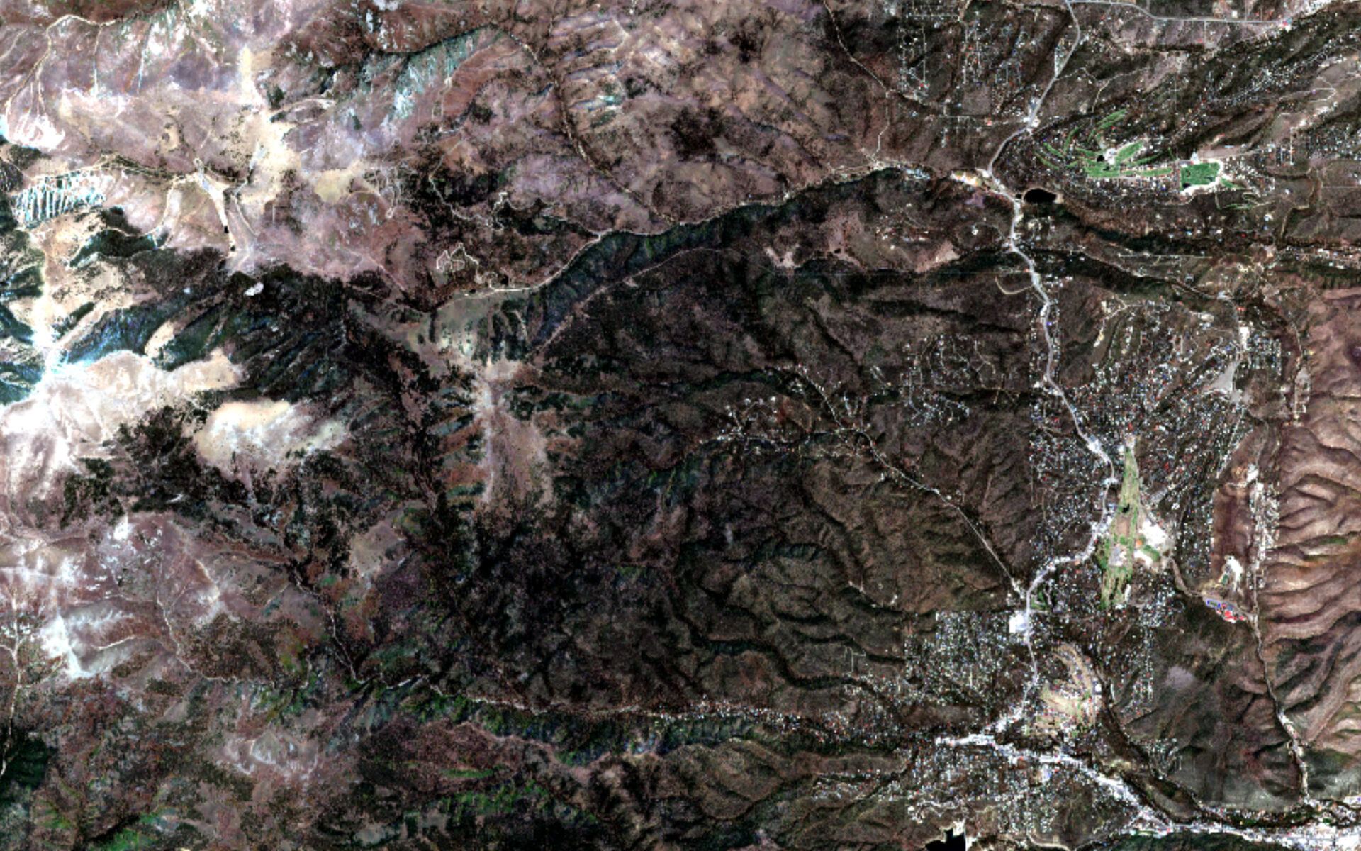
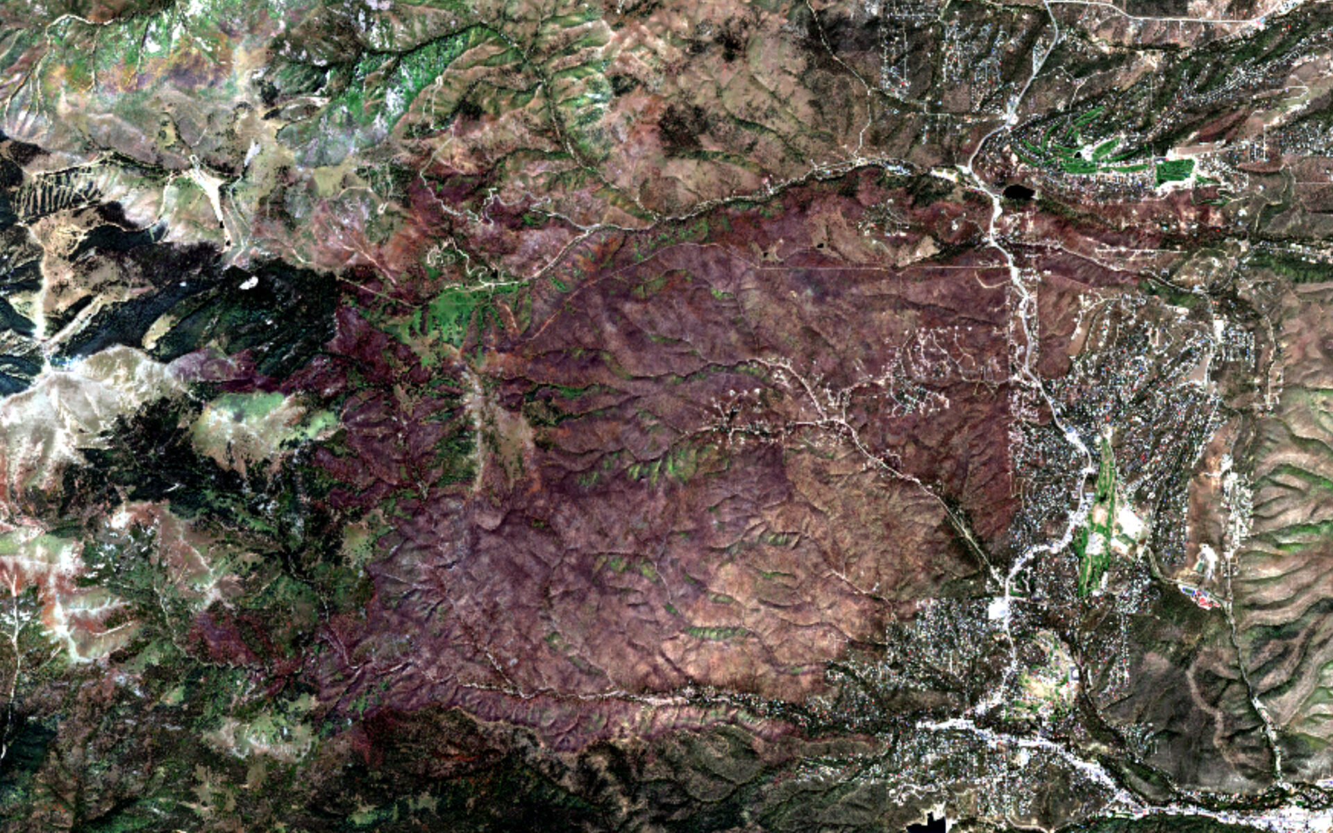
Color-infrared composites emphasize vegetation by displaying near-infrared, red, and green wavelengths. Healthy vegetation appears bright red, sparse or stressed vegetation appears pink, and burned or barren surfaces appear dark green or black.
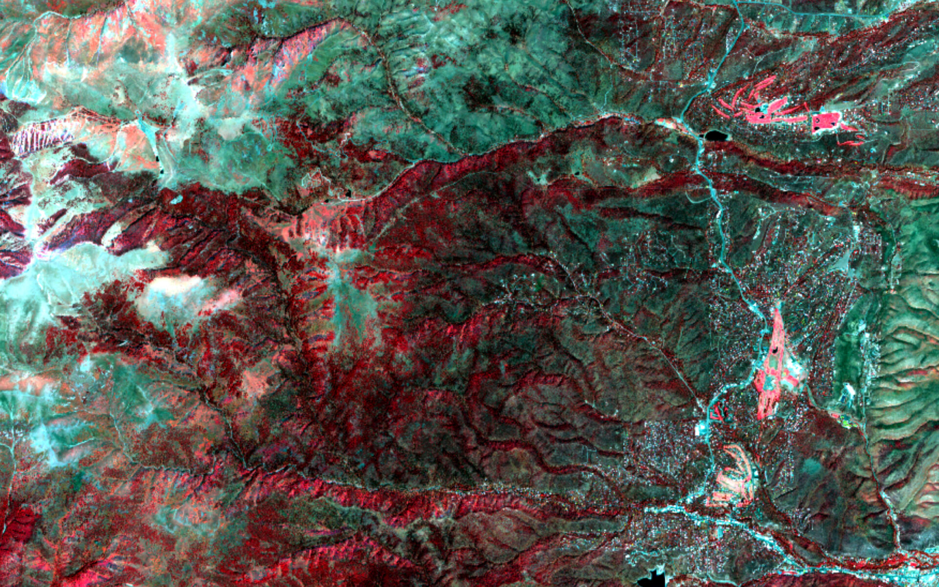
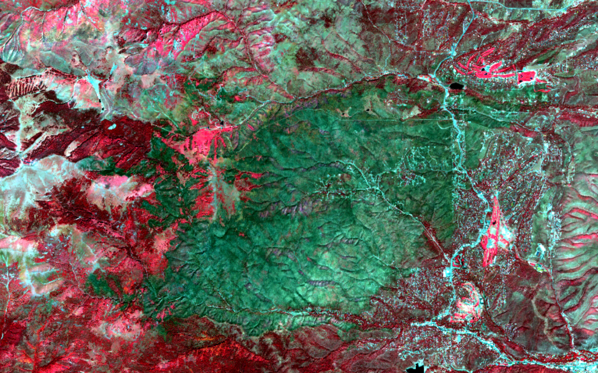
Sentinel-2 Level-2A imagery is distributed as atmospherically corrected surface reflectance, reducing the need for additional radiometric preprocessing. I did not apply a separate topographic correction. Difference-based indices can reduce the influence of persistent terrain effects, but they do not eliminate illumination differences completely; this remains a limitation of the analysis.
Translating spectral change into burn severity
Healthy vegetation strongly reflects near-infrared energy and absorbs more short-wave infrared energy. Burned surfaces generally reflect less near-infrared energy and more short-wave infrared energy than healthy vegetation. The Normalized Burn Ratio captures the contrast:
NBR = (NIR − SWIR2) / (NIR + SWIR2)
Higher positive values generally indicate denser vegetation, while lower values are more common across sparse vegetation, bare ground, water, and burned surfaces.
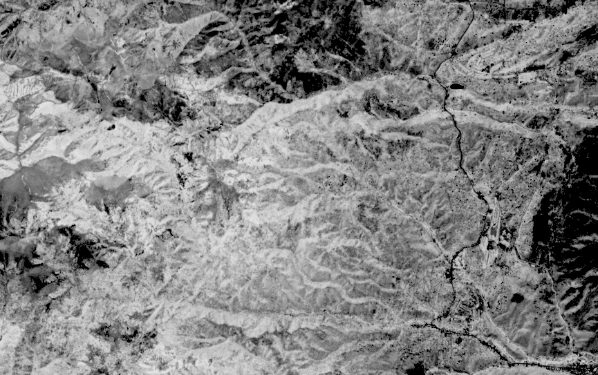

The accompanying histograms show how the overall distribution shifted after the fire.
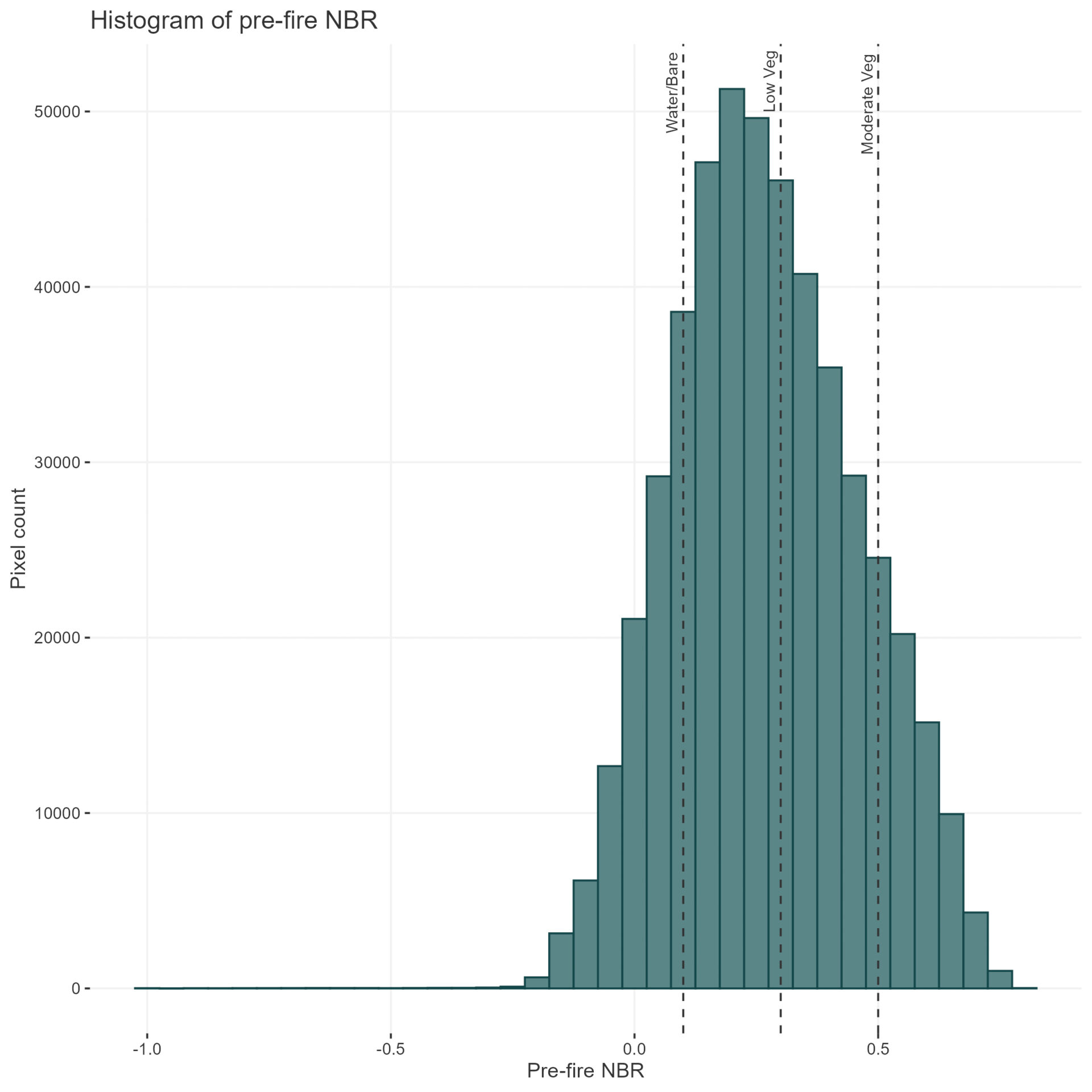

A general interpretation of NBR values is:
| NBR range | General interpretation |
|---|---|
| Less than 0.1 | Water or bare ground |
| 0.1–0.3 | Sparse vegetation |
| 0.3–0.5 | Moderate vegetation cover |
| Greater than 0.5 | Dense vegetation cover |
NBR describes conditions at one point in time. Burn severity is estimated more directly by subtracting post-fire NBR from pre-fire NBR. This differenced Normalized Burn Ratio, or dNBR, produces larger positive values where the spectral change was greatest.
Because the study area includes dense forests, open shrublands, grasslands, and developed areas, pre-fire vegetation conditions varied considerably. Relative differenced Normalized Burn Ratio, or RdNBR, adjusts dNBR according to the amount of vegetation present before the fire:
RdNBR = dNBR / √|pre-fire NBR|
This normalization makes it easier to compare relative change across a heterogeneous landscape. RdNBR values were classified using thresholds developed by Miller and Thode into unburned, low-, moderate-, and high-severity classes.


The project retained dNBR for several area summaries. Pixels with dNBR values greater than 100 were treated as burned, producing approximately 6,400 hectares of mapped burned area. Key and Benson’s dNBR thresholds then divided those pixels into low, moderate-low, moderate-high, and high severity for comparison with land cover.
Comparing fire effects across land cover
I compared ESA WorldCover with Dynamic World and selected Dynamic World because its 10-meter resolution and temporal coverage were better suited to the scale and timing of the analysis. The resulting 2024 land-cover composite was used to provide context for the mapped burn pattern.

Dynamic World is a global classification product rather than a locally validated land-cover inventory. Its categories should therefore be interpreted as broad landscape indicators. Mixed pixels and temporal variation may be especially influential in smaller classes such as water, flooded vegetation, and crops.
To compare land cover with the dNBR burn mask, I calculated the total area of each class, the area meeting the burned threshold, and the percentage of that class mapped as burned.
| Class | Total area (hectares) | Burned area (hectares) | Percent burned |
|---|---|---|---|
| Bare ground | 541.2 | 47.0 | 9% |
| Crops | 435.0 | 168.8 | 39% |
| Flooded vegetation | 139.5 | 25.2 | 18% |
| Grass | 256.7 | 23.8 | 9% |
| Shrub and scrub | 10,839.0 | 4,956.8 | 46% |
| Trees | 4,175.8 | 889.2 | 21% |
| Urban area | 3,025.8 | 315.8 | 10% |
| Water | 22.4 | 7.4 | 33% |

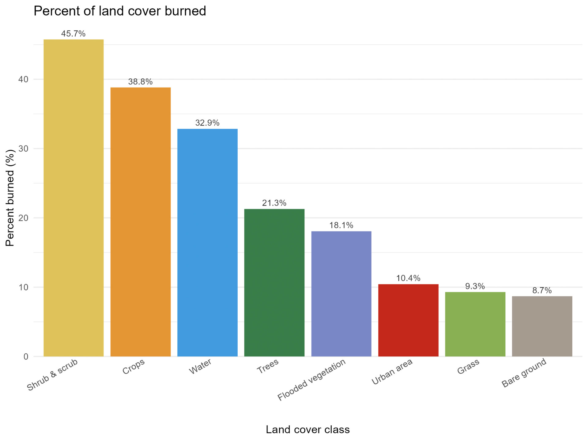
Shrub and scrub accounted for the largest mapped burned area and also had the largest burned percentage among the major land-cover classes. Approximately 21 percent of the tree class met the burned threshold. The mapped urban class had a lower percentage burned, approximately 10 percent, with most of its affected area falling within the low and moderate-low dNBR classes.
The results for smaller categories should be interpreted cautiously. For example, the comparatively high percentages reported for water and crops may reflect mixed pixels, changes in moisture, or land-cover classification uncertainty rather than straightforward burning of those surfaces.
Relating vegetation condition to burn severity
The Normalized Difference Vegetation Index, or NDVI, provides a complementary measure of vegetation greenness. Comparing pre- and post-fire NDVI helps show where photosynthetic activity declined following the fire.
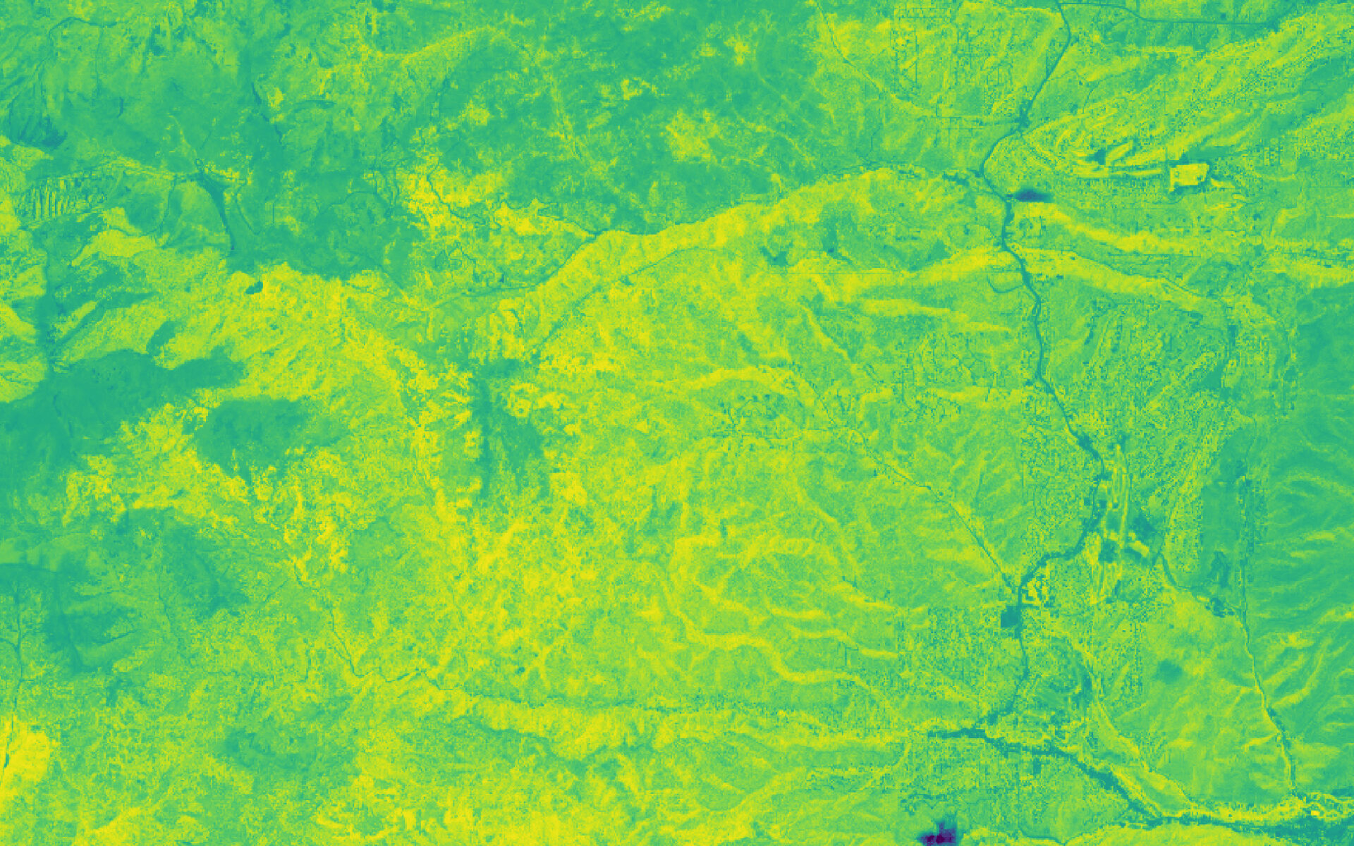

I also compared pre-fire NDVI with RdNBR to examine whether areas with greater vegetation cover tended to experience greater spectral change.

r = 0.42). Areas with greater pre-fire vegetation greenness tended to show greater relative change, although the relationship was highly variable.The correlation does not establish that denser vegetation caused more severe burning. Fire behavior also depends on weather, fuel structure, moisture, terrain, and suppression activity. The result instead suggests that pre-fire vegetation condition was one relevant component of a much more complex burn pattern.
What the burn pattern reveals
The analysis shows that the South Fork Fire produced a spatially uneven pattern of change. Shrub and scrub contributed the greatest mapped burned area, while trees represented a smaller but still substantial share. Burned pixels also extended into developed parts of the Ruidoso area, although most mapped urban overlap occurred within the lower dNBR severity classes.
Overlaying the dNBR burn mask with the Global Human Settlement Layer placed roughly 1,000 modeled residents within population grid cells intersecting mapped burned areas. This is an estimate of spatial overlap, not a count of people whose homes were damaged, who were evacuated, or who were otherwise directly affected.
The findings should be interpreted with several limitations in mind:
- Burn-severity classes were derived from spectral thresholds and were not validated with field observations.
- The pre- and post-fire composites cover different lengths of time and different seasonal windows.
- A separate topographic correction was not applied, so terrain and illumination may have influenced some spectral differences.
- Extreme RdNBR values were masked as outliers, which may have excluded some valid high-severity pixels.
- Dynamic World is a global classification product, and its local categories were not independently validated.
- The population comparison uses a modeled gridded surface rather than observed household impacts.
- The analysis captures immediate post-fire conditions and does not measure subsequent recovery.
With those limitations in view, the project demonstrates how satellite imagery can move beyond mapping a fire perimeter to reveal differences within the burn scar. Spectral indices, land-cover comparisons, statistical graphics, and cartographic design together provide an initial baseline for understanding where landscape change was greatest.
Future monitoring could compare imagery from the same season over the next one to five years. Tracking NBR and NDVI through time, incorporating slope and aspect, and comparing satellite results with field observations would help distinguish short-term spectral change from sustained ecological effects and identify areas where recovery is slow.
Citations
European Space Agency. (2015). Harmonized Sentinel-2 MSI: MultiSpectral Instrument, Level-2A surface reflectance [Data set]. Google Earth Engine.
https://developers.google.com/earth-engine/datasets/catalog/COPERNICUS_S2_SR_HARMONIZED
Federal Bureau of Investigation. (2024, July 3). South Fork Fire in New Mexico caused by lightning strike.
https://www.fbi.gov/contact-us/field-offices/albuquerque/news/south-fork-fire-in-new-mexico-caused-by-lightning-strike
Google. (2022). Dynamic World V1 [Data set]. Google Earth Engine.
https://developers.google.com/earth-engine/datasets/catalog/GOOGLE_DYNAMICWORLD_V1
Joint Research Centre. (2023). Global Human Settlement Layer population grid, 2023 release [Data set]. Google Earth Engine.
https://developers.google.com/earth-engine/datasets/catalog/JRC_GHSL_P2023A_GHS_POP
Key, C. H., & Benson, N. C. (2006). Landscape assessment: Ground measure of severity, the Normalized Burn Ratio, and remote sensing of severity, the delta Normalized Burn Ratio. In D. C. Lutes et al., FIREMON: Fire effects monitoring and inventory system. U.S. Department of Agriculture, Forest Service, Rocky Mountain Research Station.
https://www.fs.usda.gov/rm/pubs/rmrs_gtr164.pdf
Miller, J. D., & Thode, A. E. (2007). Quantifying burn severity in a heterogeneous landscape with a relative version of the delta Normalized Burn Ratio. Remote Sensing of Environment, 109(1), 66–80.
https://doi.org/10.1016/j.rse.2006.12.006
NASA. (2022). Fire Information for Resource Management System [Data set]. Google Earth Engine.
https://developers.google.com/earth-engine/datasets/catalog/FIRMS
NASA Applied Remote Sensing Training Program. (2022). Mapping burn severity using remote sensing data in Google Earth Engine [Training materials].
https://appliedsciences.nasa.gov/what-we-do/capacity-building/arset
National Interagency Fire Center. (2024). WFIGS Current Interagency Fire Perimeters [Data set].
https://data-nifc.opendata.arcgis.com/datasets/nifc::wfigs-current-interagency-fire-perimeters/about
U.S. Forest Service. (2024). South Fork and Salt fires incident information. InciWeb.
https://inciweb.wildfire.gov/incident-information/nmmea-south-fork-and-salt
U.S. Geological Survey. (2017). Monitoring Trends in Burn Severity data availability.
https://www.mtbs.gov/data-availability
World Wildlife Fund. (2006). HydroSHEDS level 10 basins [Data set]. Google Earth Engine.
https://developers.google.com/earth-engine/datasets/catalog/WWF_HydroSHEDS_v1_Basins_hybas_10
Categories: Mapping, Spatial analysis, Scripting and development, Image and remote sensing