A map becomes analytical when it moves beyond being a display and starts answering questions. An attribute query filters features according to information stored in the data table. A spatial query asks how features relate by location: what is nearby, what intersects, or what falls inside a boundary. Spatial joins then carry those relationships into a new layer, often by counting points within larger areas.
Using publicly available data for Boston, Massachusetts, this project applied those building blocks to historic resources, recreational trails, libraries, public transportation, neighborhoods, and zoning. Boston’s compact footprint and dense overlap of cultural resources and infrastructure made it a useful setting for the exercise. The individual questions vary, but the progression remains the same: filter the data, relate the layers, and map what changes.

Building the Boston dataset
Public datasets from MassGIS, the City of Boston, and the Massachusetts Bay Transportation Authority supplied the layers for the analysis. The statewide municipalities layer was filtered using TOWN = 'BOSTON' to establish the study boundary, and the remaining layers were clipped to that extent.
All source data were downloaded on July 14, 2025, and projected to NAD 1983 StatePlane Massachusetts Mainland FIPS 2001 (US Feet). This projected coordinate system limits distortion across the city and expresses the distance and area measurements used in the analysis in feet.
| Layer | Source | Feature service / dataset |
| Public libraries | Analyze Boston | Public Libraries |
| Historic inventory points | MassGIS | MassHistoric Commission Inventory |
| Hiking trails | MassGIS | Massachusetts Hiking and Wilderness Trails |
| Bicycle facilities and trails | MassGIS | Bike Trails |
| Rapid-transit lines and stations | MassGIS | MBTA Rapid Transit |
| Bus routes and stops | MassGIS | MBTA Bus Routes and Stops |
| Neighborhood boundaries | City of Boston Planning Department | Boston Neighborhood Boundaries |
| Zoning subdistricts | City of Boston Planning Department | Boston Zoning Subdistricts |
| Municipal boundary | MassGIS | Massachusetts Municipalities |
Filtering by what the data says
An attribute query works like a filter on a table: it selects map features whose stored values match a defined rule. One text query and one numeric query demonstrate how the same operation can answer very different questions.
The historic inventory contained more than 17,000 Boston records. Because the SIGNIFICAN field stores one or more descriptors for each site, a LIKE expression with wildcard characters was used to find records containing an art-related significance value:
SIGNIFICAN LIKE '%Art%'
The query selected 598 historic sites associated with art or artistic significance. Although they occur throughout Boston, the strongest clustering appears around Downtown and Beacon Hill.

A second query used a numeric field rather than descriptive text. Because trail length was stored in feet, one mile could be translated directly into a threshold of 5,280 feet:
SHAPE_Length > 5280
Ten mapped bicycle-trail features exceeded that threshold. The two longest stretches followed Dorchester Bay and crossed Franklin Park.

Defining access through distance and boundaries
Spatial queries ask how features are arranged rather than relying only on what their attributes say. A relationship might be defined by distance, intersection, or containment. The choice of relationship shapes what the result can reasonably mean.
A 500-foot distance query selected 1,764 historic sites near MBTA rapid-transit stops. The sites cluster most heavily around Downtown and along portions of the Green and Silver Line corridors. Because the distance was measured in a straight line rather than along sidewalks and street crossings, the result describes proximity to transit rather than actual walking access.

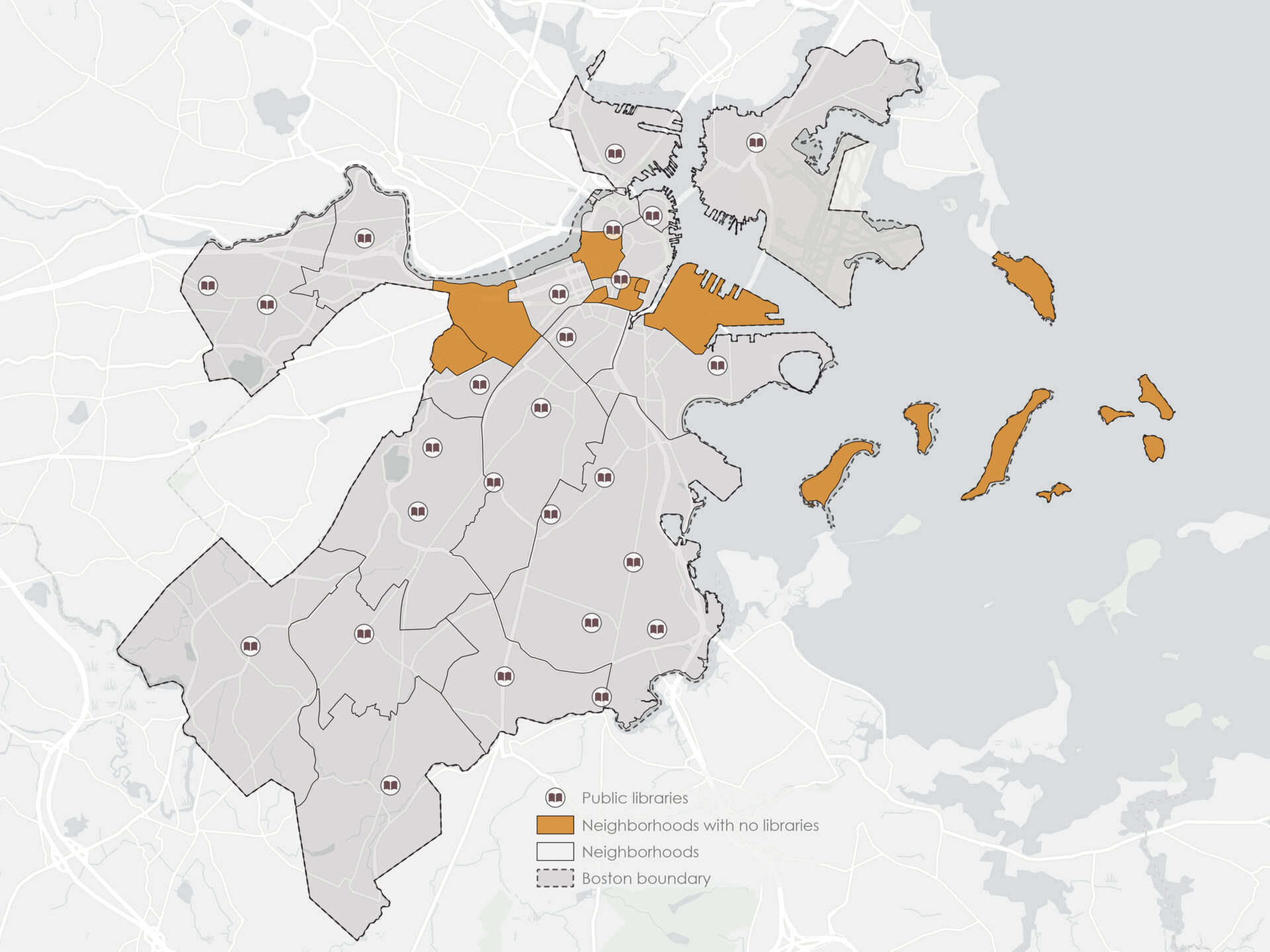
A second spatial query examined containment rather than proximity. By inverting the relationship between neighborhood polygons and public-library locations, the analysis identified eight neighborhoods without a library inside their boundaries:
- Longwood
- Bay Village
- Leather District
- Chinatown
- Beacon Hill
- Fenway
- South Boston Waterfront
- Harbor Islands
That distinction matters. A neighborhood without a branch inside its boundary may still have convenient access to one immediately across the line (with the exception of Harbor Islands). The result identifies branch absence within each neighborhood, not a complete measure of library accessibility.
Turning points into neighborhood patterns
Selections isolate individual features. Spatial joins can reorganize them into area-based summaries. By counting the points that intersect each neighborhood polygon, thousands of separate locations become neighborhood patterns that can be compared and mapped.
A spatial join of historic sites to neighborhoods found the greatest raw totals in Roxbury (2,134 sites), Dorchester (1,948 sites), and Back Bay (1,748 sites). Raw totals are partly influenced by neighborhood size, however. Once the counts were normalized by area, Back Bay, Beacon Hill, North End, and the Leather District had the highest concentrations of historic sites.
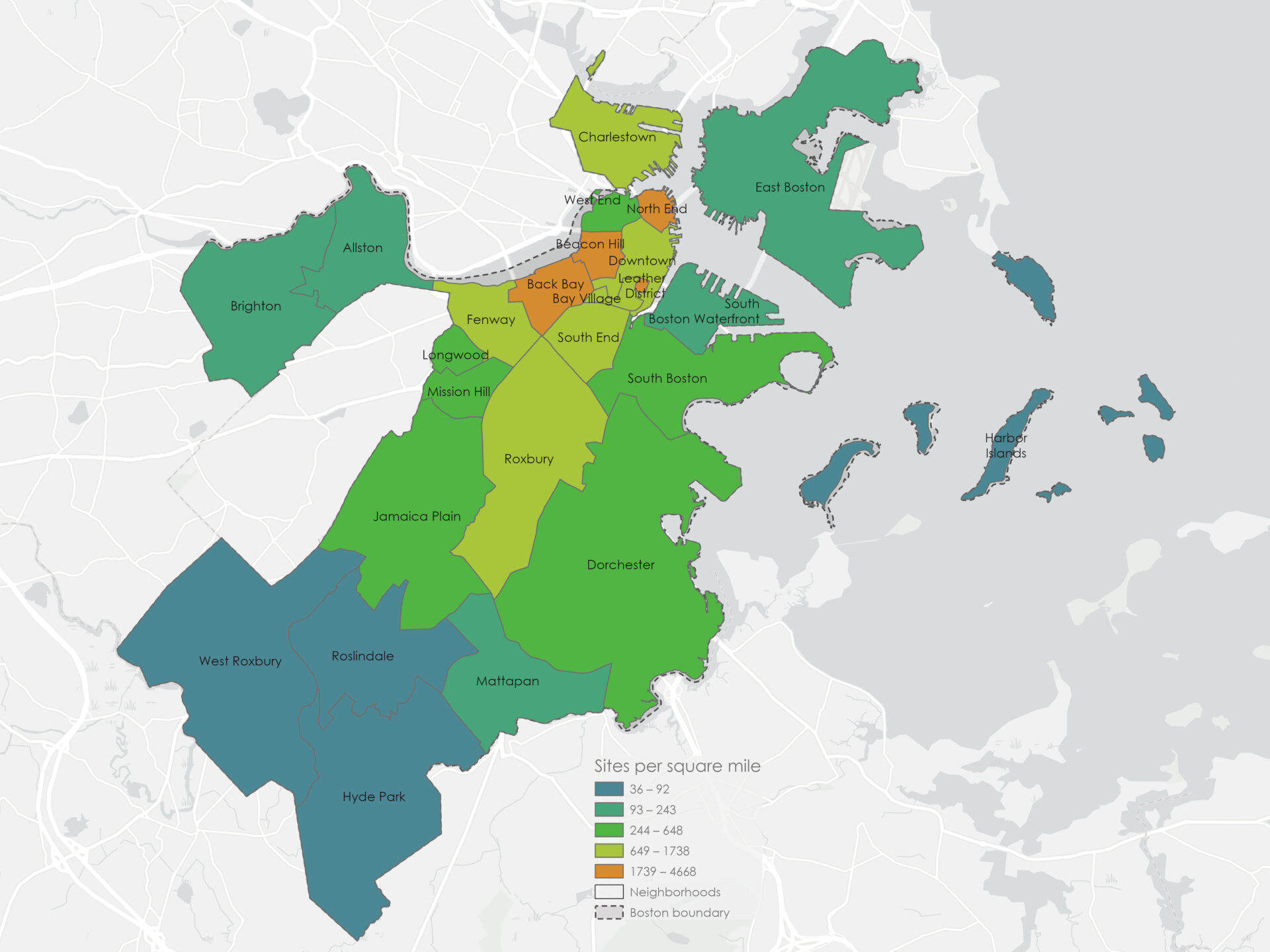
A second spatial join summarized bus stops by neighborhood. Dorchester contained the largest raw total, with 367 stops, followed by West Roxbury with 189, and Hyde Park with 168. After accounting for neighborhood area, the highest concentrations appeared around central Boston. (Harbor Islands contained no mapped stops.)
Bus-stop density indicates where stops are concentrated, but it does not describe route frequency, service hours, capacity, or the destinations those routes reach. A stop is a point on a map. Transit quality is a considerably larger question.

Layering the questions
Queries and joins become more useful when they are chained together. The final analyses combined attribute and spatial conditions to identify patterns that no individual source layer recorded directly.
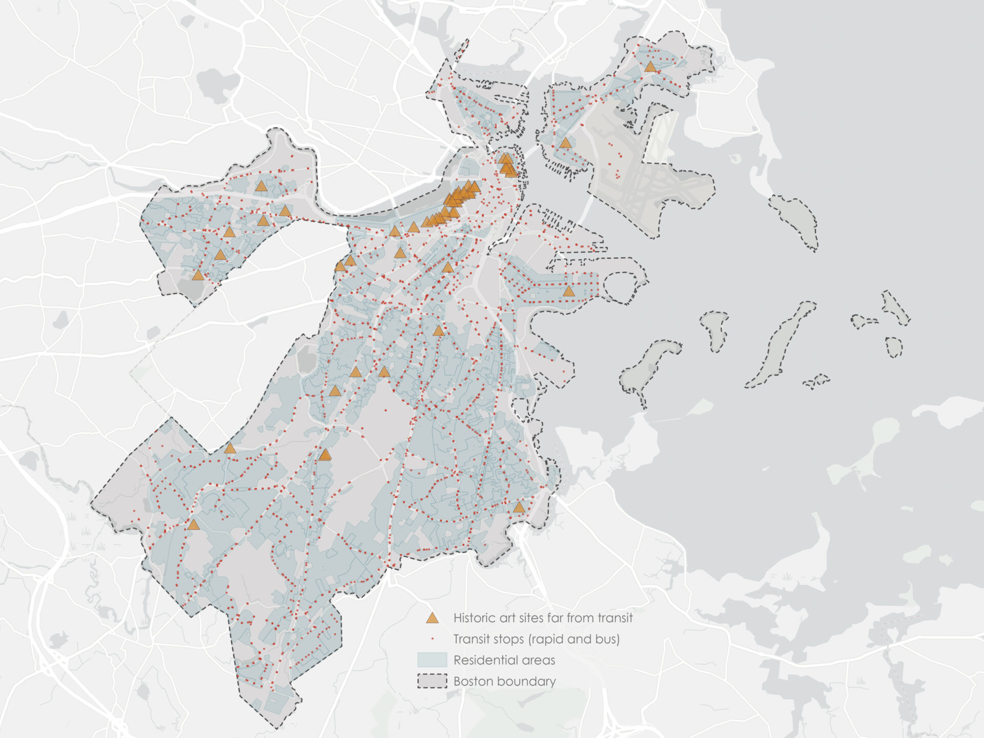
Starting with the 598 art-related historic sites, two inverted distance queries removed locations within 500 feet of either a bus stop or a rapid-transit stop. That reduced the set to 230 sites. Residential zoning polygons were then isolated using:
Subdistrict_Use LIKE '%Residential%'
Selecting the remaining sites that intersected those residential areas produced a final set of 68. Most were clustered in Back Bay and Beacon Hill, and the most transit-remote site was approximately 1,146 feet (0.2 miles) from the nearest mapped stop. (As before, those distances are straight-line measurements rather than walking routes.)
The final question combined two neighborhood summaries. Sequential spatial joins counted the hiking-trail features and rapid-transit stops intersecting each neighborhood. An attribute query then selected areas meeting both thresholds:
Trail_Count >= 100 AND Transit_Count > 5
Fenway, Roxbury, Allston, and Brighton met both conditions. The trail count represents intersecting mapped features or segments (not 100 distinct named trails) but the result still identifies neighborhoods where recreational infrastructure and rapid transit overlap particularly strongly.

What the layers reveal
None of these operations was especially complex. Their analytical power comes from sequence: attribute queries identify what matters, spatial queries introduce distance and containment, and spatial joins turn individual features into neighborhood patterns. Combining those steps produces increasingly specific questions that no source dataset could answer on its own.
The maps matter to that progression, too. A consistent extent, subdued contextual layers, and stronger color for each result allow the series to read as one investigation rather than eight unrelated exercises. The cartography makes the analytical logic visible: what was selected, what was excluded, and where the resulting pattern occurs.
The results are best read as exploratory indicators. Several limitations shape their interpretation:
- Straight-line proximity does not reproduce a walkable route or account for physical barriers.
- Feature counts and densities do not measure service quality, frequency, use, or population need.
- Boundary-based results depend on the neighborhood and zoning definitions used.
- All findings inherit the coverage, collection dates, and agency priorities of their source datasets.
Within those limits, the project demonstrates how foundational spatial-analysis methods can turn a collection of public layers into progressively sharper questions about a city.
Citations
The analytical workflow was adapted from query and spatial-join exercises in Price (2020).
City of Boston. (n.d.). Public libraries [Data set]. ArcGIS Online. https://www.arcgis.com/home/item.html?id=cb00f9248aa6404ab741071ca3806c0e
City of Boston Planning Department. (n.d.). Boston neighborhood boundaries [Data set]. ArcGIS Online. https://www.arcgis.com/home/item.html?id=fefd5fb156d9419e80a3944a62bd64ab
City of Boston Planning Department. (n.d.). Boston zoning subdistricts [Data set]. ArcGIS Online. https://www.arcgis.com/home/item.html?id=fffb5de90c814daabf2cfd5538b8d22c
Massachusetts Historical Commission. (n.d.). MassHistoric Commission inventory [Data set]. MassGIS. https://www.arcgis.com/home/item.html?id=e27a15d822ef4b10bb4dd6eb631ceb3c
MassGIS. (n.d.). Bike trails [Data set]. ArcGIS Online. https://www.arcgis.com/home/item.html?id=f3ced38395ab4d5a8b5e7568c7bf8b5d
MassGIS. (n.d.). Massachusetts hiking and wilderness trails [Data set]. ArcGIS Online. https://www.arcgis.com/home/item.html?id=7c6ff96b59e2493797c9cdcc2135c61a
MassGIS. (n.d.). Massachusetts municipalities with generalized coast [Data set]. ArcGIS Online. https://www.arcgis.com/home/item.html?id=54538f2f92d04c34957e6c2d460d0e5a
MassGIS. (n.d.). MBTA bus routes and stops [Data set]. ArcGIS Online. https://www.arcgis.com/home/item.html?id=86e2b8d6fcf94ee2832dbb6758ee03d5
MassGIS. (n.d.). MBTA rapid transit [Data set]. ArcGIS Online. https://www.arcgis.com/home/item.html?id=dba3f84748654013a04d24dcfe3725be
Price, M. H. (2020). Mastering ArcGIS Pro. McGraw-Hill Education.
Categories: Mapping, Spatial analysis