Fine particulate matter (PM2.5) refers to fine particulate matter with a diameter of 2.5 micrometers or smaller. These particles are small enough to be inhaled deeply into the lungs and can pose serious health risks.
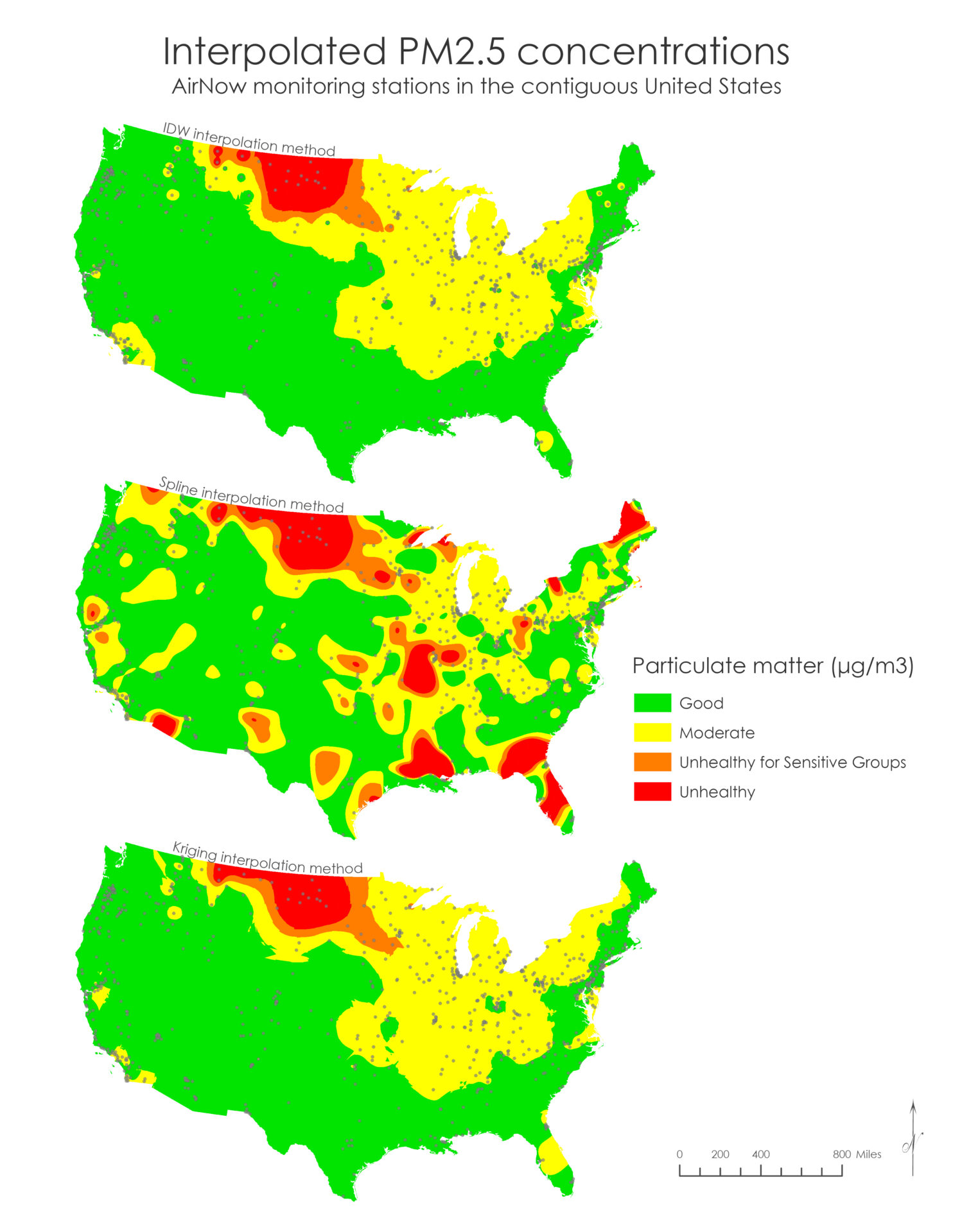
This project applied spatial interpolation methods to estimate PM2.5 concentrations at unsampled locations using publicly available EPA AirNow data in order to determine which method — Inverse Distance Weighted (IDW), Spline, or Kriging — most accurately predicted PM2.5 concentrations across the contiguous U.S.
Study area
The study area for this analysis was the contiguous United States, which includes the 48 adjoining U.S. states and excludes Alaska, Hawaii, and U.S. territories. This region spans a wide range of geographic and climatic conditions, from coastal zones to mountain ranges and major urban centers.
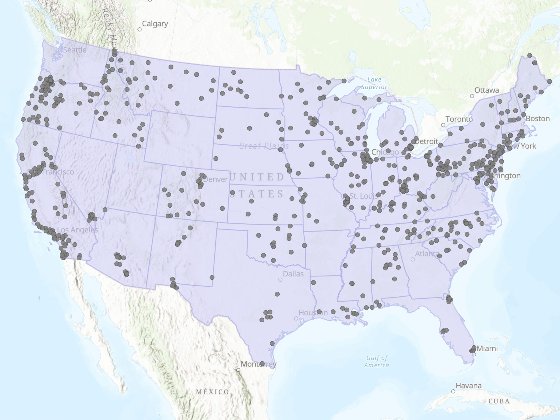
The extent was defined by a generalized U.S. state boundaries dataset used to mask and constrain interpolated output surfaces.
Data
The PM2.5 data used in this project came from the EPA’s AirNow Air Quality Monitoring Site Data (Current) feature service, which provides near-real-time air quality observations from EPA-affiliated ground-based monitoring stations. The dataset included point features with pollutant readings, including raw concentration values for fine particulate matter (PM2.5).
The PM2.5 values in this dataset represent hourly concentrations of fine particulate matter measured in micrograms per cubic meter (µg/m³). For more information about PM2.5 and its health impacts, see the U.S. Environmental Protection Agency’s PM basics page.
All layers were projected to NAD 1983 Contiguous USA Albers (EPSG:5070), an equal-area projection optimized for U.S.-scale spatial analysis. This projection preserves area and supports accurate interpolation by ensuring consistent distance and spatial relationships between points.
The AirNow dataset included readings from monitoring stations located in multiple countries, including some outside the United States.
| Dataset | AirNow Air Quality Monitoring Site Data (Current) |
| Year of publication | Updated continuously (accessed June 11, 2025) |
| Owner | US EPA, Office of Air and Radiation, Office of Air Quality Planning and Standards (OAQPS) |
| URL | AirNow feature service |
| Description | Provides current air quality values and AQI scores for pollutants measured at EPA monitoring sites, including PM2.5, PM10, and ozone. |
| Coordinate system | NAD 1983 Contiguous USA Albers (EPSG: 5070); Geodetic Datum: North American Datum 1983 (NAD83) |
| Geometry Type | Point (vector) |
Data filtering
To focus the analysis on the contiguous U.S., I created a filtered layer based on the StateName field that includes only stations within the lower 48 states and Washington, D.C. The following SQL expression was used to select those records:
StateName IN (
  'AL', 'AZ', 'AR', 'CA', 'CO', 'CT', 'DE', 'FL', 'GA',
  'ID', 'IL', 'IN', 'IA', 'KS', 'KY', 'LA', 'ME', 'MD',
  'MA', 'MI', 'MN', 'MS', 'MO', 'MT', 'NE', 'NV', 'NH',
  'NJ', 'NM', 'NY', 'NC', 'ND', 'OH', 'OK', 'OR', 'PA',
  'RI', 'SC', 'SD', 'TN', 'TX', 'UT', 'VT', 'VA', 'WA',
  'WV', 'WI', 'WY', 'DC'
)
The original dataset contained 4,392 records representing air quality monitoring stations. To focus the analysis on relevant and reliable observations, the following station filtering rules were applied:
- Stations located within the lower 48 states and Washington, D.C. (based on the StateName field).
- Status = “Active”
- PM2.5 IS NOT NULL
- PM25 >= 0
After these steps, the final dataset used for interpolation included 746 monitoring sites, each representing a unique location with valid PM2.5 data.
Training and test sets
To evaluate the performance of the IDW, Spline, and Kriging interpolation methods, the dataset was split into training and test subsets:
- The training set (90%), consisting of 671 points, was used to generate the interpolation surfaces.
- The test set (10%), consisting of 75 points, was held out to assess the accuracy of each method.
Interpolation methods
Three spatial interpolation methods were used to estimate PM2.5 concentrations from the training data: IDW, Spline, and Kriging.
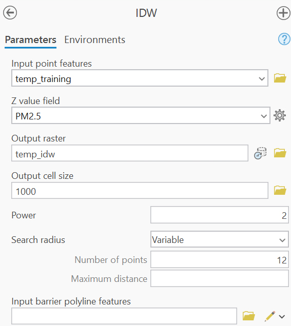
Inverse Distance Weighted (IDW)
Inverse Distance Weighted (IDW) interpolation estimates unknown values based on nearby measured values, with closer points having more influence than distant ones.
A power value of 2 was used with a variable search radius limited to the 12 nearest neighbors, reflecting a standard assumption that closer points have more influence on prediction.

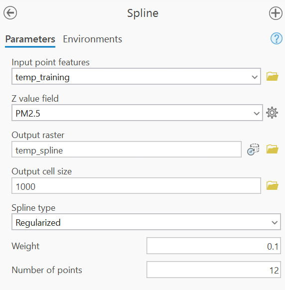
Spline
Spline interpolation fits a smooth surface through the measured values by minimizing surface curvature.
Spline interpolation was run using the Regularized option with a weight of 0.1 and the same neighbor settings to produce a smooth, continuous surface.
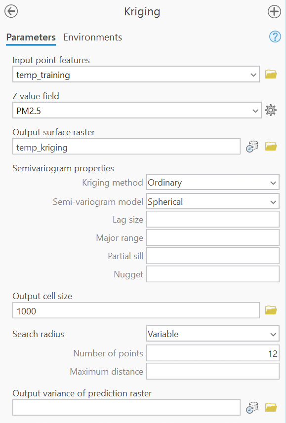
Kriging
Kriging is a geostatistical interpolation method that accounts for both the distance and spatial autocorrelation between measured points.
Kriging was performed using Ordinary Kriging with a spherical semivariogram model, again using 12 neighbors and a variable search radius.
All three interpolation outputs were then symbolized following the EPA’s published PM2.5 breakpoints for Air Quality Index (AQI) categories (pages 8–9):
| AQI Category | PM2.5 Range (µg/m³) |
|---|---|
| Good | 0.0 – 12.0 |
| Moderate | 12.1 – 35.4 |
| Unhealthy for Sensitive Groups | 35.5 – 55.4 |
| Unhealthy | 55.5 – 150.4 |
| Very Unhealthy | 150.5 – 250.4 |
| Hazardous | 250.5+ |
Results
Since the maximum value in the dataset was 131 µg/m³, only the first four categories (Good through Unhealthy) were utilized in the classified rasters.
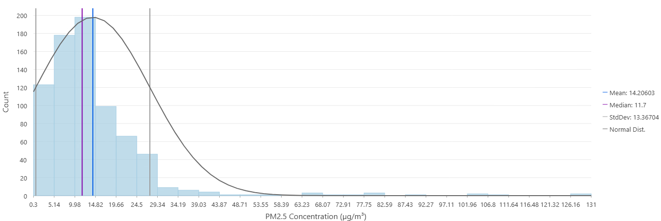
The table below compares summary statistics from each interpolation surface to the original observed PM2.5 values to assess how well the methods represent the overall data distribution.
| Method | Minimum | Maximum | Mean | Standard Deviation |
|---|---|---|---|---|
| Observed points | 0.30 | 131 | 14.21 | 13.37 |
| IDW | 0.31 | 131 | 14.52 | 15.54 |
| Spline | -1,027.58 | 271 | 11.38 | 46.11 |
| Kriging | 0.35 | 131 | 13.76 | 15.09 |
In order to evaluate the interpolation performance compared to the observed points, I computed the following four accuracy metrics from the 75 test points:
- Mean Absolute Error (MAE)
- Mean Squared Error (MSE)
- Root Mean Squared Error (RMSE)
- R²
| Interpolation method | Mean Absolute Error (MAE) | Mean Squared Error (MSE) | Root Mean Square Error (RMSE) | R² |
|---|---|---|---|---|
| Inverse Distance Weighted (IDW) | 3.74 | 56.28 | 7.50 | 0.78 |
| Spline | 14.01 | 2198.53 | 46.89 | -7.63 |
| Kriging | 3.50 | 38.39 | 6.20 | 0.85 |
Conclusion
Kriging produced the best overall results, with the lowest RMSE (6.20 µg/m³) and the highest R² (0.85), indicating strong predictive accuracy and spatial coherence. This is clearly the method that would best predict missing values for this dataset.
IDW performed slightly worse, with an RMSE of 7.50 and R² of 0.78.
Spline performed poorly, with a much higher RMSE (46.89) and a strongly negative R² (–7.63), suggesting that, for this data, the method performed worse than simply using the mean.
A key limitation of this analysis is the uneven spatial distribution of the monitoring stations across the U.S. Coverage appears to be densest in urban and highly populated areas, while large regions are sparsely monitored or entirely unrepresented.
In this dataset, there were no active stations in the following states:
- Arkansas
- Georgia
- Massachusetts
- Utah
- Virginia
- Washington
- Wyoming
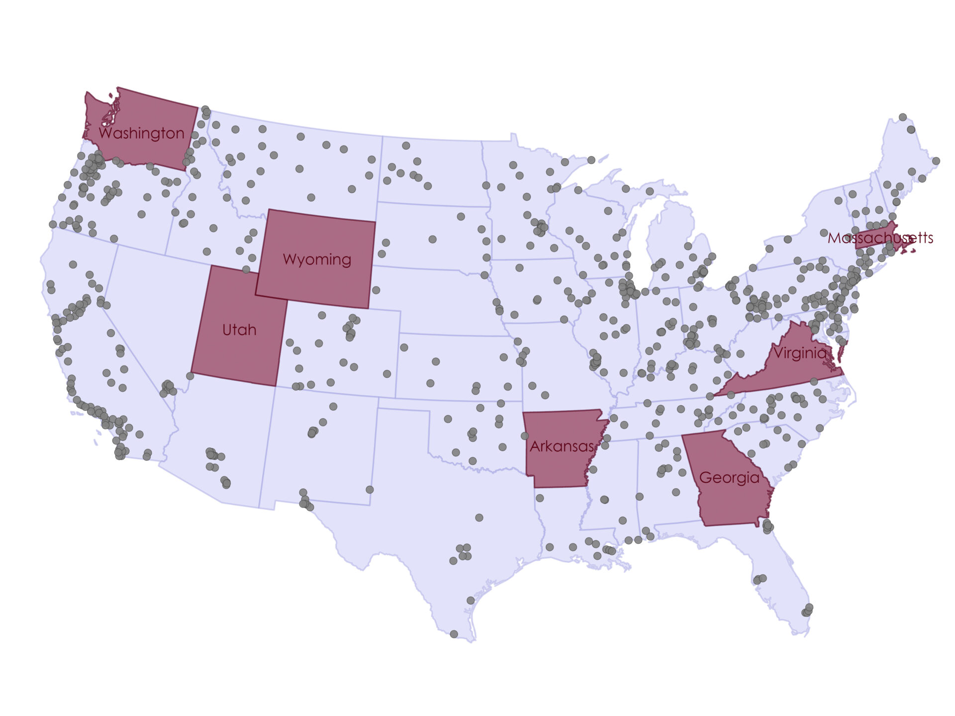
This spatial imbalance may introduce interpolation bias, particularly in rural or data-scarce areas, where estimates rely on distant training points and may therefore be less reliable.